
08 Oct Alts and the Bell Curve
By QP Wealth Management
October 8, 2020
We often get asked why we use alternative investments and I like to think we have a simple and effective way of demonstrating our answer. Imagery is powerful teaching tool, so the bell curve lends itself nicely to our method. If you have never seen a bell curve here is an introduction. In brief, it is a tool for measuring risk/reward probability. In order to use the bell curve to explain the advantage of alts, we need to make a comparison to other asset classes.
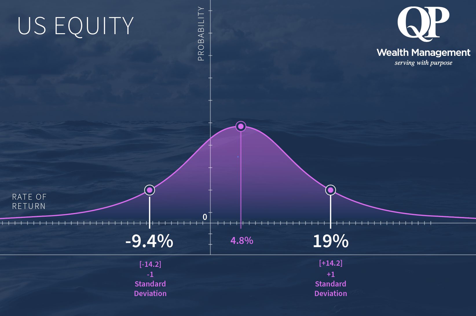
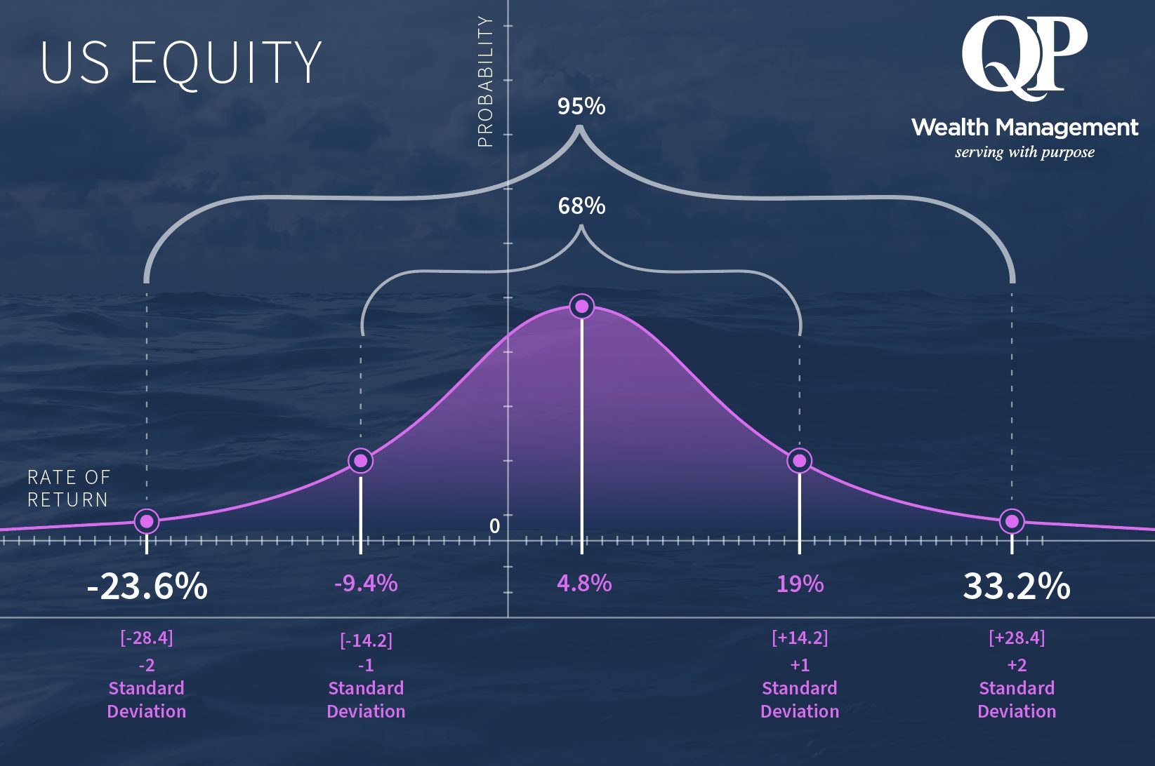
Let’s start with demonstrating equities, in this case we will use US equities. We’ll have to make an assumption as to our rate of return and the kind of volatility we face as equity investors. For this exercise we’ve taken our assumptions from Morgan Stanley’s Global Investment Committee. This provides that our rate of return for the next seven years would be approximately 4.8%. And with that we should be willing to accept about 14.2% annualized volatility – also referred to as standard deviation.
To depict this on a bell curve we have our rate of return on the bottom axis, and we draw a normal bell curve above. Our expected annual return of 4.8% (or mean) placed in the center of the bottom axis in line with the peak of the bell.

The volatility, or standard deviation, is depicted by two lines drawn at equal intervals (up and down) from our 4.8% return. These lines are +1 standard deviation and -1 standard deviation from the mean. To solve for the return expected at each standard deviation we add/subtract our volatility (14.2%) from the mean (4.8%). This means that 19% is our return at 1 standard deviation up from the mean and -9.4% is what we should expect at 1 standard deviation down from the mean. Now, how does that translate into something meaningful for the investor?
At one standard deviation (between -1 and +1) we can expect 68% of our results. So, 68% of the time our returns will fall between -9.4% and 19%. To increase the probability of capturing results you should also assess return expectations at two standard deviations. To solve for this, you would add and subtract 2x volatility (28.4%) from the mean. This gives us a return of -23.6% and 33.2% at two standard deviations. This represents that 95% of the time, our returns will fall between -23.6% and 33.2%. Experience tells us investors are apt to be complacent when results fall to the right of the mean but become uncomfortable when faced with returns to the left. Additionally, the farther left you go the more likely you are to see kneejerk decision-making.
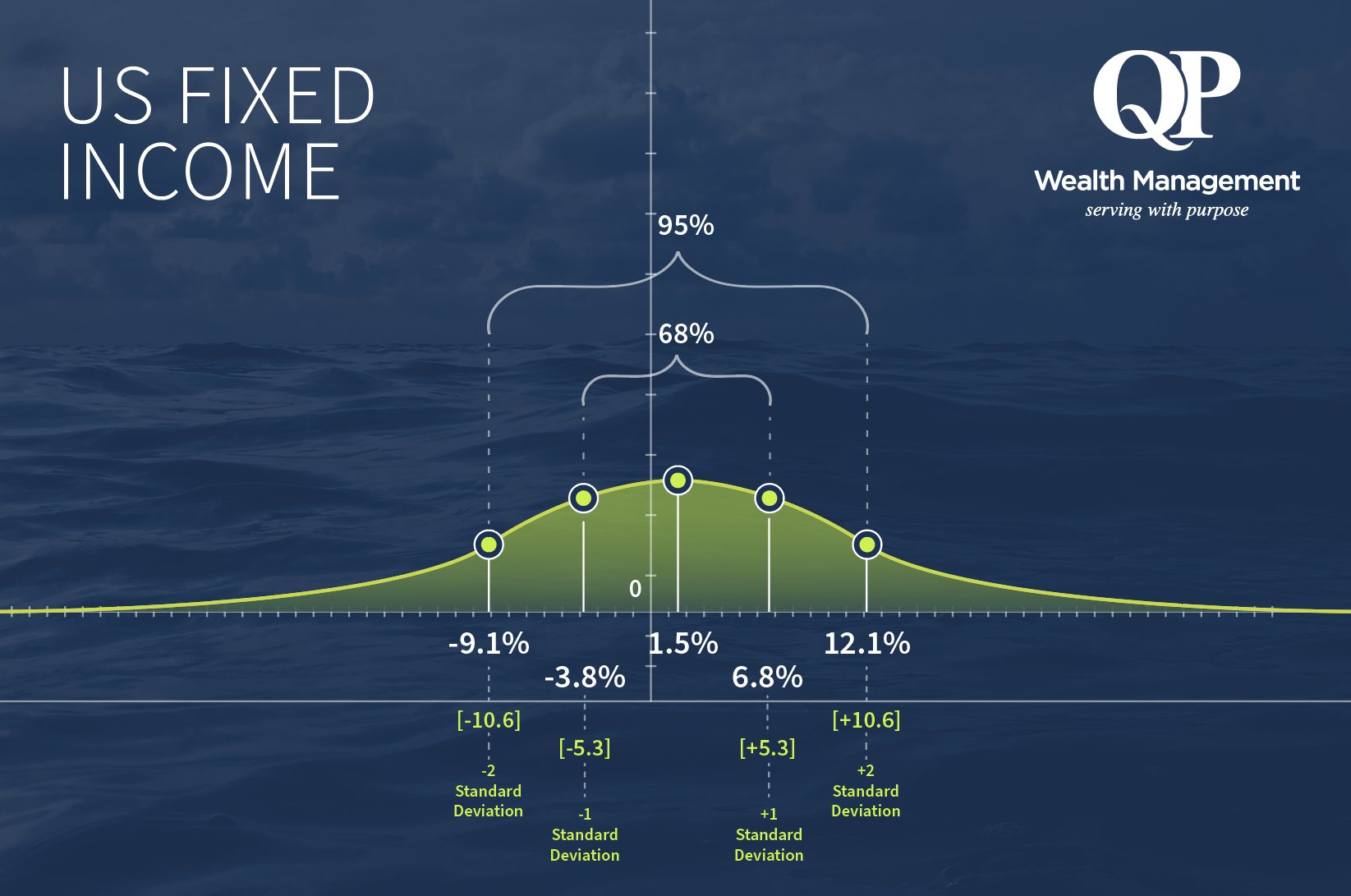
But how can you reduce the likelihood that your results fall to the left of the mean? The most traditional answer is fixed income. US fixed income, specifically, is projected to have a 1.5% rate of return over the next seven years with a 5.3% standard deviation. At +1 standard deviation you would have returns of 6.8% and at -1 standard deviation you will have -3.8%. Going out two standard deviations you will have 12.1% and -9.1%. As you can see in the image below, this asset class shrinks the area of your return results. In this case, the price of less volatility is the size of your reward.
This brings us to alternative investments. For the last scenario, we’ll use private real estate, just one of many alternative investment classes. The return assumption is 8.5% for the next seven years with an annualized volatility of 8.4%. At +1 standard deviation we land at 16.9% and -1 standard deviation we have .1% (still positive).

Let’s just compare those numbers to our equity and fixed income scenario. 68% of the time your returns will fall between .1% and 16.9%. At two standard deviations, 95% of your results will fall between -8.3% and 25.3%. Interpreting these assumptions through the bell curve paints a meaningful picture for investors. This tool demonstrates private real estate achieving fixed income-like volatility with equity-like returns.

Investors should always use a mix of asset classes to optimize an appropriate risk/reward ratio. But in constructing that mix you tend to sacrifice one for the other. “QPers” with access to alternative investments have a competitive advantage in portfolio building. Keep in mind, alts can be complex, illiquid, and require high minimums to participate. Moreover, there are various types of alternative investments and while we used private real estate to demonstrate this point, each has unique features which translate differently on the bell curve. These are all factors that should be weighed when determining which and how much to allocate. My point is simply that they should be considered, when suitable, as a component to potentially increase returns, decrease risk, or both as a part of an overall portfolio.
QP Wealth Management is an investment advisor. Information presented is for educational purposes only. Past performance is not indicative of future performance. Principal value and investment return will fluctuate. There are no implied guarantees or assurances that the target returns will be achieved or objectives will be met. Future returns may differ significantly from past returns due to many different factors. Investments involve risk and the possibility of loss of principal. The information used in this report were obtained from sources Morgan Stanley. Please let us know if you have any questions.